CrossRef API

Searching for scientific articles using an API (application programming interface) allows you to extract data from publisher platforms and databases. With an API, you can create programmatic searches of a citation database, extract statistical data, or query and manipulate your results within a Notebook.

In this module, we will learn to use the Crossref API to search for and analyze scientific articles.

What is Crossref?¶

Crossref is a non-profit organization that helps to provides access to scientific literature. Crossref “makes research outputs easy to find, cite, link, and assess” (https://www.crossref.org/).

Crossref data on scientific publications essentially consists of three elements:
1) Metadata about a publication
2) A URL link to the article
3) A document identifier (doi)

At present Crossref contains information on 80 million scientific publications including articles, books and book chapters.

Installing Packages¶

First we will install packages that will be useful to us as we explore the Crossref API. When importing a package into Jupyter Notebook, we use the command pip install ... to download a package into Jupyter Notebook.

We then use the command import (package name) to use our new package in our code.

Analysis using Crossref API¶

In the sections below, we will walk through the basics of Crossref.

Data can be accessed using the python packages habanero, crossrefapi, and crossref-commons installed above. In this , we’ll be focusing on the functionality of the habanero package.

Exploring a Crossref query¶

In the cells below, we walk through using Crossref and exploring the data it gives us. To create an object that takes on the Crossref identity, we assign it to the variable cr.

The main function we will use is called cr.works(). This function takes in a query name. As an example, we’ll use the search term “permafrost”.

In order to save this output, we’ll assign it to the variable name permafrost.

If we inspect permafrost, we can see that it is a dictionary. A dictionary is a type of data structure that is indexed by keys.

In the cell below, try creating your own query for a different search term. Make sure to save it to a variable! For now, limit your search term to a single word.

Keys, Indexes, Metadata¶

A dictionary contains key-value pairs, and we can access the values by calling on the keys. In our permafrost dictionary, we can inspect the keys and take a look at the values that it contains.

Above, we can see that there are 4 different keys in our permafrost dictionary. We will focus on the values for the message key. In the cell below, we are accessing the values by indexing into the dictionary by the given keys.

This dictionary is nested, meaning that we can have keys that lead to values which are more dictionaries. It seems like the message contains most of the information we’re interested in. Below, take a look at the keys of the message component of the permafrost dictionary.

Just as we did before, we can inspect what information is contained for different keys of the dictionary. Let’s focus on total results first.

Above, we can see that the items contains the majority of information about our query on permafrost. It contains a list of all of the results - we can check this with the type command we used earlier. Since we only are looking at the first page, our items list has only 20 items in it.

Creating Tables¶

When our data exists in dictionaries, it’s a little hard to explore and manipulate. In order to tackle this, we’ll create a dataframe of the information so that we can access it more easily.

There are a bunch of columns in our table, and we can’t see all of them by scrolling. Below, we can look at a list of the columns instead.

Container-title seems to stand in for Journal Title. Let’s look at what’s in the container title column:

We can do the same for the publisher column.

Data Retrieval¶

We want to be able to retrieve more data from CrossRef. A single CrossRef query can return up to 1,000 results, and since our query has over 42,000 total results, we would need to make 43 queries. Remember at the beginning, we only had 20 results since we only grabbed the first page. The CrossRef API permits fetching results from multiple pages, so by setting cursor to * and cursor_max to 1000 we can grab 1000 queries at once. Querying all 42,000 results would take a long time, so for the purposes of this demonstration we are only using 1000. If you have more time, you could query more results, but be aware that it will take a long time.

We can check that we have the 1,000 messages, and indeed we do.

Remember before, when you created your own search query? Here, we’ll go through a few steps to get more results for your query. First, we’ll check how many total results your query has. Run the cell below to find out.

If there are fewer than 1000 results, then set cursor_max to the number of results. If there are more than 1000 results, set cursor_max to 1000 so that the code won’t take too long to run. Be sure to fill in query with the same search term you used earlier.

In order to get all of the different results from our permafrost query, we need to extract them from cr_permafrost. Below, we create a list where each element is one result. cr_permafrost is a list consisting of pages, where we have 20 results per page. So cr_permafrost has 50 pages of 20 results each, giving us our 1000 results. In order to extract the info and have a list with each element be one results, we need to do some data manipulation.

In the cell below, we have 2 list comprehensions to get the results from our query. The first one creates a length 50 list that contains only the items instead of the entire dictionary, for each of the 50 pages. The second list comprehension extracts all of the items from the nested lists so that we have a single 1000 item list where each element is one result.

We’ll do the same for your query results so that you can have some fun plotting later in the notebook. Just uncomment and run the cell below.

More on Searches¶

You may be curious about the cr.works function that we’ve been using to get our data. This is the function that processes your topical “search”. There are different arguments, and we’ve seen how changing these arguments can help us get more search results than just the first 20.

Also, before we asked you to limit your search term to a single word. This is not a hard restriction - we simply did this for simplicity. You can query terms that are more specific and include more words - try it out below! Keep in mind that the more specific your search query, the fewer results you may see. Feel free to play around with it.

Visualization¶

Visualization is an important part of data analysis. Rather than looking at dictionaries and dataframes, we can see a visual summary of our data. In this section, we’ll go over different types of visualizations we can make based off of the different data we have. We’ll start by looking at the publishers. But first, we need to do some wrangling to get the data in a form that’s useful for us.

Grouping and Sorting by Journal¶

In an earlier section, we took our query results and converted them from a dictionary to a dataframe. Below, we will do this for our list of 1000 permafrost_items, and then we can use the dataframe methods of grouping and sorting to get the counts of articles published by each publisher. We can also group by other columns, such as type or language.

In the cell below, we create a dataframe containing all 1000 of our permafrost query results.

While we are at it, we’ll convert your search query items into a data frame as well. Adapt the code in the cell to create a dataframe out of your query_items list.

Counts¶

We can take the value_count to determine the number of times a given journal or work appears in our results. This will help us determine where research on our topic is commonly published.

The journal dataframe above shows us that we have about 300 different titles, and a lot of them published only a few articles. The journal that appears most often published about 130 articles on our topic.

Bar Charts¶

Now that we have a sorted dataframe with journal titles and the number of articles they each published on permafrost, we can use this dataframe to plot the journals with the 10 highest counts.

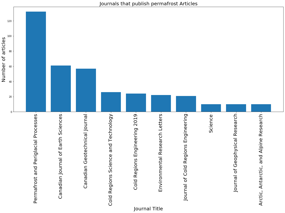
Before, we grouped by journal title. Keep in mind that we can group by other tags as well, such as type of article (type) or the language the article was published in (language). In the cell below, we use another method to group by either type or language and plot the resulting bar chart. Remember to sort your dataframe as well.

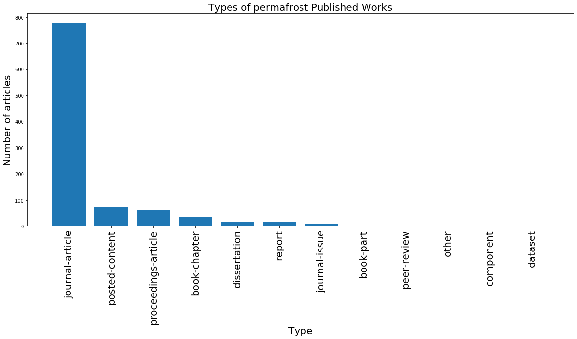
If you’d like, you can use the cells below to create bar charts of publisher, language, or type for your own query by grouping and sorting your query_df dataframe! Feel free to reference the cells above for an example with permafrost_df.

Citations¶

In scientific literature, we are often also interested in the number of references a journal article has, or the number of times the article was cited. Let’s see which articles have been cited the most - we can do this by sorting our dataframe by the is-referenced-by-count column. Our dataframe has 45 columns, but we’ll just focus on a few. We’ll look at the title, is-referenced-by-count, publisher, and published-print (the date it was published in print).

Let’s look at the top 10 most cited articles.

What is the most cited article, and when was it published? Do you think the date it was published has an effect on the number of times the article was referenced?

Replace this line with your answer

Visualizing the Number of Citations¶

When looking at our most_cited table, we can see that the most number of times an article was referenced was 181, and the least was 0. Using a type of visualization called a histogram, we can look at the distribution of time an article was referenced. We’ll do this in the cell below.

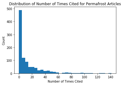
We can see that this histogram is very skewed, with the majority of articles being cited fewer than 50 times. We can adjust the bins in order to see a better distribution, by specifying the sizes of the bins.

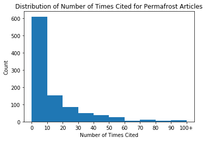
In the cells below, we’ve provided code to look at the number of times each article was cited for your query_df. In the following cell, try applying what you’ve just used to find the most cited article, the date it was published, and create a histogram showing the distribution for all articles.

Queries Over Time¶

For our final visualization, we will look at 2 queries over time. To expand our searches to 2 words, we will look at queries for permafrost melt and arctic methane, and look at the number of articles that were published by year. Since running queries takes a long time, and ideally we want to have more years to compare over time, we pre-ran the queries and saved the results into a csv which we’ll load in the cell below.

The following 8 cells show the code we used to generate the csv files.

Below, we’ll load in our query data and extract the year from the created column. Since we read in our data from a csv, our created column got converted to strings instead of dictionaries. We use the function ast.literal_eval() in order to convert the string back to a dictionary, and then access the year by indexing into date-parts.

In the cell below, we create a plot comparing the number of articles published for glacier melt and for permafrost melt per year. For year_counts_glacier and year_counts_permafrost, we use the python package Counter to return the counts of articles for each year. We sort by year so that our plot follows sequentially.

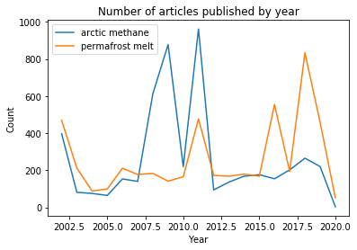
Our search results show a spike in articles related to methane in the arctic in 2008 and 2011, and a later set of spikes for articles about permafrost melt between 2016-2019. We would have to dig in a bit more to understand the implications of these peaks, but they do give you a place to start when exploring trending topics.

If you are interested, you could repeat the process of getting queries and edit the above code to compare two search terms that you are interested about.

Bibliography ¶

• Paul Oldham - Adapted CrossRef R guide to Python. https://poldham.github.io/abs/crossref.html#introduction

Notebook originally developed by: Keilyn Yuzuki, Anjali Unnithan

This chapter originated as a Data Science Module: http://data.berkeley.edu/education/modules